2. Obstacle Detection and Slope Estimation

2.1. Road Extraction

Using the disparity map, we identify the road profile using v-disparity and u-disparity maps as per the method proposed by Wu, Meiqing, Chengju Zhou, and Thambipillai Srikanthan in Nonparametric Technique Based High-Speed Road Surface Detection at IEEE Transactions on Intelligent Transportation Systems. The method can provide road approximations even for non-planar road surfaces as well.

First, based on the disparity map u-disparity map is generated. The peaks in the u-disparity map corresponds to the obstacles. So the u-disparity map in then applied to thresholding to identify the peak and thus the disparity values corresponding to the obstacles. This step is there to help with road profile extraction by removing large obstacles which will otherwise lead to erronous results in road profile. You can either use a constant as a threshold or use a threshold depending on the disparity value which is the better choice as objects that are far away corresponds to smaller number of pixels in the image. Thus threshold values are pre-calculated based on the equation below.

(2.6)\[\begin{equation} u\_threshold(d) = \frac{minHeight\times d}{b} \end{equation}\]

where \(b\) is the baseline, \(d\) is disparity and \(minHeight\) is the minimum height if the obstacle you need to consider as a large obstacle. We keep the minimum height as 0.4 m.

Once you detect the peaks in the u-disparity, the corresponding obstacle can be easily removed from the original disparity map. Then the v-disparity map is generated from this large obstacle removed disparity map. Road surface can be obtained with v-disparity. It is done based on several observations, (1) maximum intensity value in at least first few rows belongs to the road (i.e. bottom part of the image will mostly constitute from the road), (2) in adjacent rows the disparity value of the road in the higher row (smaller row number)is always smaller than or equal to disparity value of the road in the lower row (higher row number). Road profile extraction is started from the bottom of the image. Based on the first assumption the detection process is initiated by identifying the highest intensity of the v-disparity map for the first few rows. Then road profile is approximated by traversing row by row based on the second assumption. For this purpose we first construct an initial road profile by just sorting the disparity value corresponding to the peak intensity value for each row of the v-disparity map. Then if the disparity value of the peak intensity of the row in consideration is equal or lower than (within a threshold limit to avoid outliers) that is of the previous row, that disparity is added to the disparity road profile. If no match found the same disparity as per previous row is considered. Then you finish the process once you observe that the road profile is not moving to the left for a threshold number of rows.

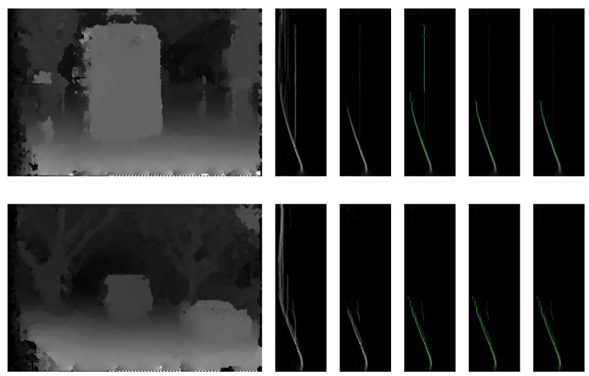
Fig. 2.5 Road profile extraction process. Left to right: Initial v-disparity, Large obstacles removed v-disparity, Peak points of the v-disparity (in green), Road profile (in green)

Each row of the original disparity image is checked with the corresponding disparity value from the road profile. If the disparity \(d_i(r,i)\) is less than the corresponding disparity from the road disparity profile \(d_{rp}(r)\) plus a pre-defined small threshold value \(d_{th}\), that pixel in the rectified image is assigned as a road pixel \(p_{road}\) otherwise an obstacle pixel \(p_{obs}\). That is, pixel \(p \in p_{road}\) if \(d_i(r,i) < (d_{rp}(r) + d_{th})\) or \(p \in p_{obs}\) otherwise. Then for \(p \in p_{road}\) for which \(d_i(r,i) > (d_{rp}(r)\), \(p\) is checked whether it was identified as a large obstacle in the u-disparity based method, if yes \(p\) is re-assigned to \(p \in p_{obs}\). Small threshold \(d_{th}\) is required because there are some road pixels that have higher disparity value than the median road disparity value. These pixels \(p \in p_{obs}\) are then analysed to find a meaningful obstacle segmentation.

2.2. Positive Obstacle Detection

Method proposed by Meiqing Wu, Student Member, Chengju Zhou, Thambipillai Srikanthan in Robust and Low Complexity Obstacle Detection and Tracking Far and High Region at IEEE International Conference on Intelligent Transportation Systems was used.

Firstly, the pixels \(p \in p_{obs}\) are refined by removing the pixels whose 3D points are 2.5 m above the camera rig and 15 m to the left and right sides from the left camera point. The method is based on u-disparity map peaks where a new u-disparity map is generated based on an updated disparity map which only contains disparity values for refined obstacle pixel set. Every line segment in this u-disparity map corresponds to an obstacle in the image. Hysteresis type thresholding is used to remove the noise in the u-disparity image. High threshold based on (2.6) and low threshold as a ratio of high threshold is defined to compensate for different object scales due o different depths. Then all the pixels in the u-disparity is categorized into three segments as pixels above high threshold, below low thresold and between high and low thresholds. All pixels below low threshold are ignored considering them as noise and pixels above high threshold are selected. Other pixels between high and low thresholds are marked as noise if there is no single pixel in the 8-connected neighbourhood that belongs to a pixel above the high threshold, otherwise they are selected as well. Then a connected component analysis is performed based on \(u\_span\) which is a segment of connected line in the thresholded u-disparity map. Then based on a neighbourhood window all the :math:`u_span`s within that window are clustered together to single segment. Then bounding boxes are generated for these segments, where left and right boundaries are directly found from the two columns of the segments in the thresholded u-disparity map. Lower band is detected from the row corresponding to maximum disparity value in the segmentation referred from the road profile, where as upper band is detected by scanning the area bounded by other three bounds correspoding to the disparity range in the segmentation in the thresholded u-disparity image. As an additional constraint minimum number of pixels are defined to qualify that bounding box as an obstacle.

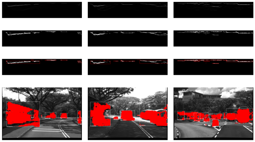
Fig. 2.6 Obstacle bounding box generating process. Top to bottom: u-disparity for refined obstacle points, Thresholded u-disparity, Segmented u-disparity, Bonding boxes detected

2.3. Negative Obstacle Detection

Based on the road profile, a region of interest is defined for the road region. Then correspoding disparity_roi and image_roi is extracted. Then two methods are proposed;

SaliencyBasedDetection – Using saliency detection on the super pixel segmented road and thresholding. This work was motivated by the observation that negative obstacles are dark compared to the other parts of the road. On the road image_roi we first perfom superpixel segmentation to cluster pixels with similar intensity values together. Superpixels segmentation method by J. Yao, M. Boben, S. Fidler, and R. Urtasun in Real-time coarse-to-fine topologically preserving segmentation at Proceedings of the IEEE Computer Society Conference on Computer Vision and Pattern Recognition. Superpixel segmentation is to reduce the computation time without needing to work on every pixel. Then based on the intensity values we identify dark regions in the road and categorise them as netaive obstacles by first thresholding and then using a cost function to identify which regions are darker compared to others.

IntensityBasedDetection – This method is based on 3D data from disparity and intensity threshold image on the road image_roi. This method was motivated by the fact that the disparity values inside a negative obstacle are smaller than the disparity values on the road which lines in the same image image row. In this method first a thresholded image based on intensity is used to find the dark regions and disparity information is used on top of that to verify that the detection is a negative obstacle.

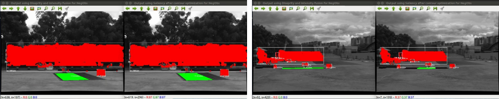
Fig. 2.7 Negative obstacle detection. Left: SaliencyBasedDetection and Right: IntensityBasedDetection

2.4. Road Slope Estimation

We make use of stereo information to calculate the road height and use this information in calculating the slope. This is also based on the road profile. Slope is calculated for three road segments with relative to the vehicle position. When the road is not visible slope is not calculated. Road not visible part are identified if the v-disparity has lower value than a threshold. We have also incorporated IMU data to detect humps and raised zebra crossing to avoid sudden jumps in the slope. Based on the road height slope is calculated following basic trigonometry. Slope angle corresponds tangential angle between the height difference of the road point to the road height of the current position and depth of the point.

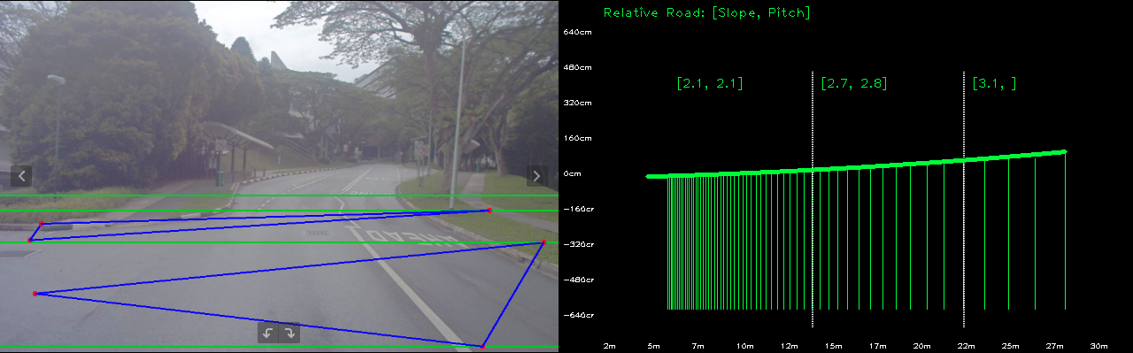
Fig. 2.8 Slope angle and pitch angle calculation in different road segments.

2.5. Road Pitch Estimation

For each road segment, surface normal to the road is calculated. Surface normal can be calculated using the cross product of two vectors that lie on the plane. Therefore, we randomly select three points in the each road segments that not collinear and take the cross prodct between the two vetors for the three points to calculated the surface normal. Once the surface normal is calculated, pitch angle of that road segment is calculated by taking the angle difference between surface normal and n vector towards perfect upward vector. Result of such pitch angle is shown in Fig. 2.8.